Understanding AlphaGenome, Part 2: The Architecture, The Model and What It Can Do
U-Net DNA, teacher–student distillation, 5,930 tracks, GWAS to T-ALL: how AlphaGenome compresses a megabase, attends globally and scores variants, plus how to run it.
Imagine you're a geneticist and a patient hands you a result.
A genome-wide association study has flagged a variant as statistically associated with type 2 diabetes across hundreds of thousands of people. This is real signal. The statistics are airtight.
You have no idea what it means.
The variant is non-coding. There's no protein consequence to compute. The nearest eQTL database didn't sample pancreatic beta cells, which are the cells that actually matter for diabetes. The variant has never been functionally characterized in any laboratory. And running an experiment for every variant in every GWAS, at the scale of modern genetics, is simply not possible.
This is where most variant interpretation pipelines hit a wall.
AlphaGenome's central claim is that it can take that variant's DNA sequence, just the letters and predict what biology would look like across gene expression, splicing, chromatin accessibility, histone marks, transcription factor binding and 3D genome contacts simultaneously, across thousands of cell types and tissues. The variant doesn't need to have been measured in any lab. The model doesn't need prior knowledge of that locus.
It predicts from scratch. And then Part 2 is about whether you should believe it.
The Architecture: Compress, Process, Expand
Part 1 covered the biology and the tension: you need to see a 500 kb regulatory landscape and resolve a 6 bp binding motif at the same time and no model before AlphaGenome could do both. Part 2 is about how AlphaGenome actually solves it: the architecture, the training and what it found in a leukemia patient's genome. (New here? Start with Part 1: The Biology and the Problem.)
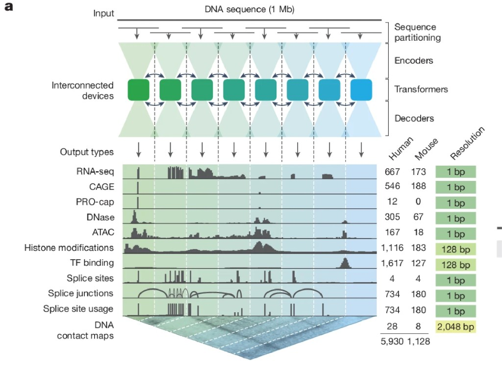
Fig 1a: architecture and output routing
Part 1 ended with a problem. CNNs detect local sequence patterns. Transformers communicate long-range interactions. But you can't just stack them naively, running a transformer at single-nucleotide resolution across 1 million base pairs is computationally impossible.
AlphaGenome's solution borrows a structure from medical imaging: the U-Net.
Think about what a radiologist needs to do with a chest X-ray. She needs to understand the whole picture, where the lungs sit relative to the heart, the overall density distribution and she needs to resolve a 3 mm nodule in the lower right lobe. Zoom out too far and you miss the nodule. Zoom in too close and you lose the anatomical context.
Medical image segmentation models solved this with a compress-then-expand architecture. You downsample the image until it's small enough to process at the global scale, then upsample back to full resolution, carrying fine-grained detail forward through "skip connections" that bridge each compression level to its corresponding expansion level.
AlphaGenome applies this logic to DNA.
The model takes 1 megabase of sequence and runs it through a CNN encoder that compresses it through successive downsampling steps, halving resolution at each stage. Each layer captures increasingly abstract patterns: raw nucleotide motifs first, then regulatory element signatures, then broader domain structure. By the time the sequence reaches the transformer, it's been compressed into a manageable representation where each position encodes rich local context.
The transformer runs at this compressed bottleneck. At this scale, global self-attention is feasible and the model can learn that an enhancer 200 kb away is relevant to a particular promoter, that CTCF sites at specific positions demarcate chromatin domain boundaries, that two distant positions are co-regulated.
Then the CNN decoder mirrors the encoder in reverse, upsampling back toward base-pair resolution. And here's where the skip connections matter.
Without them, the decoder would have to reconstruct nucleotide-level precision from a blurry compressed representation, like trying to restore a high-resolution photograph from a thumbnail. The skip connections carry fine-grained detail from each encoder layer directly to its corresponding decoder layer. When the decoder is reconstructing resolution X, it receives exactly what the encoder saw at resolution X.
The result: a model that has seen the whole 1 Mb regulatory landscape and retained single-nucleotide precision. The tradeoff Part 1 described isn't evaded. It's structurally dissolved.
The outputs split into two streams. Predictions about individual positions, RNA-seq, ATAC-seq, splice sites, histone marks, come out as 1D tracks at 1 bp or 128 bp resolution. Predictions about how pairs of positions relate to each other in 3D space come out as 2D contact maps at 2,048 bp resolution. Eleven modalities total. 5,930 experimental tracks across human and mouse.
One practical note on hardware: processing 1 million bases through a transformer requires distributing the work. AlphaGenome uses sequence parallelism, splitting the 1 Mb input into 131 kb chunks across 8 TPUs simultaneously, with the transformer layers communicating between devices during attention computation. Every chunk can effectively see every other chunk. The whole genome window is processed in parallel. A single variant scored across all 5,930 tracks takes under a second on an H100.
Two Training Stages: The Part Most Users Skip
This is the most important thing to understand before you trust the model's variant scores.
Think about what it takes to train someone to grade essays.
In stage one, you give them 10,000 essays with real grades. They study the patterns, this kind of writing gets an A, this gets a C. After enough examples, they get good at grading essays they've never seen. This is pre-training.
Now you ask them: "if I change one word in this essay, does the grade change?" Sometimes they say yes, sometimes no, inconsistently. Because during training they only ever saw complete essays with real grades. They learned to recognize patterns in whole documents, not to respond consistently to small perturbations.
To fix this, you freeze the expert grader, they don't learn anymore and train a new student. But instead of learning from real grades, the student learns to match whatever the expert outputs, including on essays with words swapped, sentences changed, deliberate errors introduced. The student becomes very consistent when handling small changes because it practiced handling small changes explicitly.
In AlphaGenome's terms: essays are DNA sequences, real grades are experimental data (RNA-seq, ATAC-seq, ChIP-seq), the expert is the teacher model, word changes are DNA mutations and the consistent student is the distilled model you actually run.
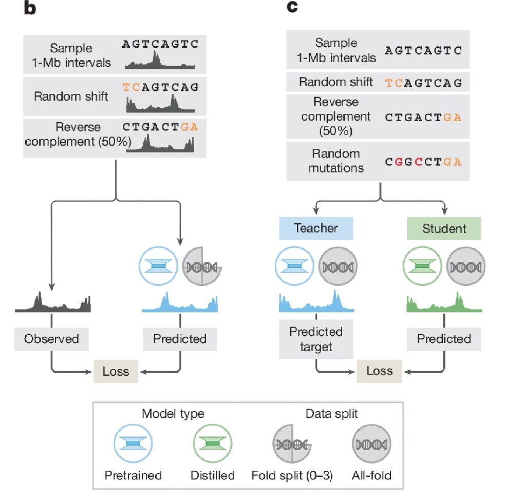
Fig 1b + 1c: pre-training and distillation side by side
Why does this matter? The teacher model was trained purely on reference genome sequences against real experimental data. It never saw mutated sequences. When you give it a variant to score, reference sequence in, alternative sequence in, subtract the outputs, the difference can be noisy. The teacher sometimes overreacts to a benign change, sometimes underreacts to a damaging one.
The distilled student has practiced millions of mutations. It has learned: when one letter changes here, the output should change by this much; when one letter changes there, the output is stable. The result is a model that responds smoothly and consistently to sequence perturbations.
The ablation studies show distillation improves variant scoring by 12–20% across all modalities. It's not a minor optimization, it accounts for a substantial fraction of AlphaGenome's advantage over previous models. And practically: one forward pass on the reference sequence, one on the alternative, subtract, you have variant effect scores across all 5,930 tracks simultaneously.
What the Model Outputs: A Routing Guide
Before running AlphaGenome, you need to know which outputs map to your question. The right output depends entirely on what you're trying to learn.
| If your question involves... | Use this output | Resolution |
|---|---|---|
| Gene expression levels | RNA-seq tracks | 1 bp |
| Where transcription starts | CAGE / PRO-cap | 1 bp |
| Exon-intron boundaries | Splice site donor/acceptor | 1 bp |
| Splice site competition | Splice site usage | 1 bp |
| Which exons connect to which | Splice junction coordinates | 1 bp |
| Open chromatin / enhancer activity | ATAC-seq, DNase-seq | 1 bp |
| Active enhancer marks | H3K27ac, H3K4me3 ChIP-seq | 128 bp |
| TF occupancy | TF ChIP-seq | 128 bp |
| 3D genome organization | Contact maps (Hi-C) | 2,048 bp |
The resolution differences are biologically motivated, not arbitrary. A splice site is a single base pair, 128 bp bins would make splice site prediction meaningless. Contact maps operate at the scale of topological domains spanning hundreds of kilobases, 2,048 bp resolution is appropriate and 1 bp would add no information. The ablation studies confirm this directly: going from 1 bp to 32 bp resolution drops splice site prediction performance from auPRC 0.79 to 0.51, essentially destroying it, while the impact on contact map prediction is minimal.
The 1D versus 2D split also matters practically. "What does this variant do to chromatin accessibility at position X?" is a 1D question, you want the ATAC-seq track. "Does this variant disrupt a chromatin loop between position X and position Y?" is a 2D question, you want the contact map. These are different biological questions requiring different model outputs.
Does It Actually Predict Real Biology?
Before trusting variant scores, you want to know the model can predict experimental measurements on sequences it has never seen.
On held-out genomic regions, predicted tracks closely mirror observed ones across six different assay types simultaneously. Peaks appear in the same places. Valleys in the same places. The contact map's triangular structure is reproduced. Mean Pearson correlations run 0.86 for splice junctions, 0.85–0.87 for ATAC and DNase, 0.79 for contact maps and 0.59–0.78 for RNA-seq depending on resolution.
Performance is consistent across human and mouse, suggesting the model has learned general regulatory principles rather than memorizing human-specific patterns.
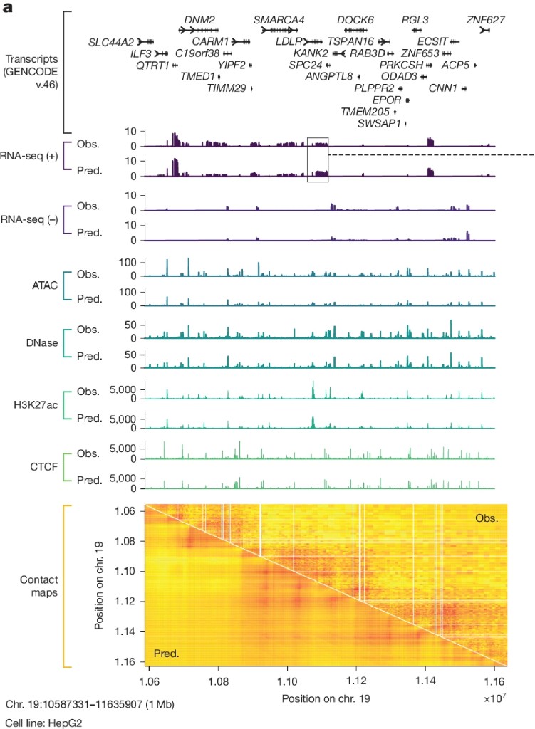
Fig 2a: 1 Mb HepG2 track comparison
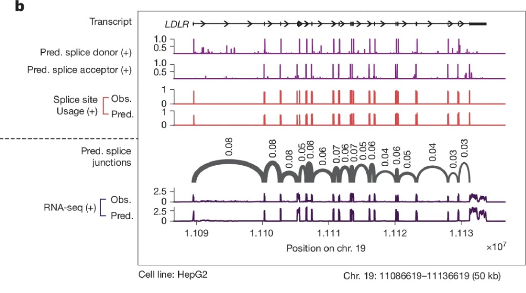
Fig 2b: LDLR splice site zoom
The splice site predictions are particularly striking. The model predicts not just where splice sites are, but how strongly they compete with each other and which donor-acceptor pairs form functional junctions. This matters clinically: many genetic diseases are caused by variants that shift splice site usage rather than eliminating a site entirely. Those subtle effects were invisible to coarser models. At 1 bp resolution, they're not.
Variant Effect Prediction: How It Works
The scoring mechanism is conceptually simple, which is part of what makes it powerful.
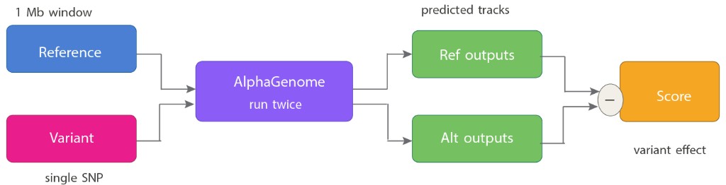
Variant effect score = Predicted tracks (alt) − Predicted tracks (ref)No lab experiment. No patient cohort. Just the letters.
The key design choice is what you do with the difference. For gene expression effects, you sum the RNA-seq track difference over the entire gene body, this captures enhancer effects from anywhere in the 1 Mb window, not just at the promoter. For chromatin accessibility, you look at the signal in a small window centered on the variant itself, since chromatin accessibility is local. For splicing, you take the maximum difference in splice site signal across all relevant positions. Each scoring strategy reflects the biology of how that modality responds to sequence change.
A concrete example. A single A→C change at rs9610445 on chromosome 22 is associated with lower APOL4 expression in colon tissue across GTEx donors. AlphaGenome correctly predicts that the C allele reduces RNA-seq signal over APOL4. Running in silico mutagenesis, systematically testing every possible single-base change at surrounding positions, reveals why: the C allele disrupts a transcription factor binding motif. The mechanistic chain runs: variant breaks TF binding site → TF can't bind → enhancer less active → less gene expression. AlphaGenome recovered that chain from DNA sequence alone.
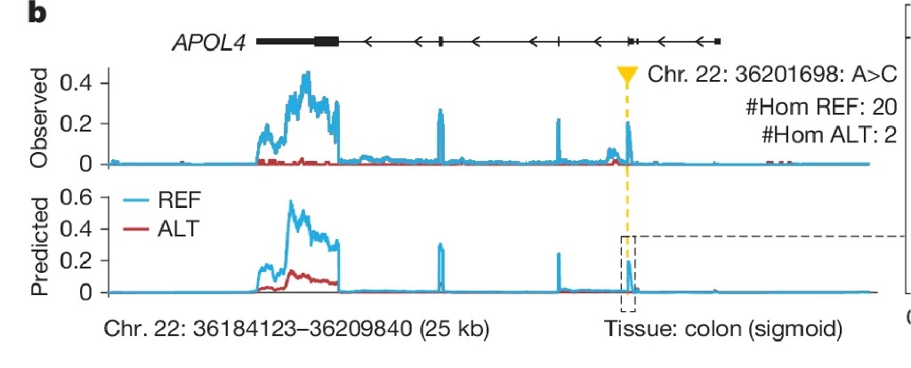
Fig 4b: APOL4, colon (sigmoid)
The TAL1 Case Study: What This Looks Like for a Real Disease
The benchmarks tell you AlphaGenome is state of the art. The TAL1 case study tells you what that actually means.
T-cell Acute Lymphoblastic Leukemia, T-ALL, is an aggressive blood cancer. In many patients, it's driven by a specific type of non-coding mutation: small insertions, just a few extra base pairs, in the regulatory region 7.5 kb upstream of a gene called TAL1. TAL1 is a transcription factor that should be silenced in mature T-cells. These insertions switch it back on. Uncontrolled proliferation follows.
Figuring out the mechanism took a research group years of laboratory work.
AlphaGenome was given one of these insertions, a two-letter change at chr1:47239296, with no prior knowledge of TAL1's regulatory biology. What it predicted:
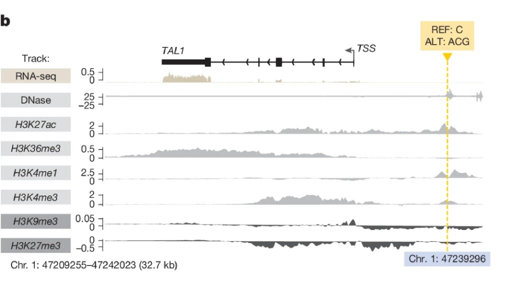
Fig 6b: TAL1 insertion predictions
Chromatin opens at the insertion site. An active enhancer mark appears. TAL1 expression increases 7.5 kb away.
All three effects. Simultaneously. From sequence alone.
But the multimodal framing is what makes the result genuinely useful rather than impressive. When you score all known T-ALL oncogenic insertions and compare them to random length-matched insertions, the oncogenic mutations consistently light up across multiple modalities at once. Background mutations scatter around zero. If you looked at only chromatin accessibility, you'd miss some oncogenic variants. Looking across all modalities simultaneously, the class of disease-causing mutations stands out clearly.
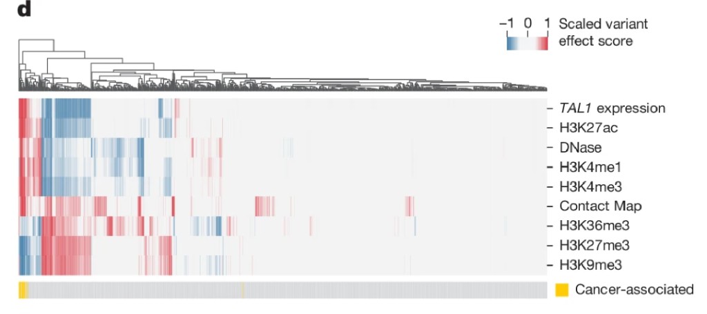
Fig 6d: multimodal heatmap
Running in silico mutagenesis on the insertion sequence reveals the mechanism: the two inserted letters create a perfect MYB transcription factor binding motif from scratch. MYB is a known oncogenic TF in leukemia. The mechanistic chain is now complete.
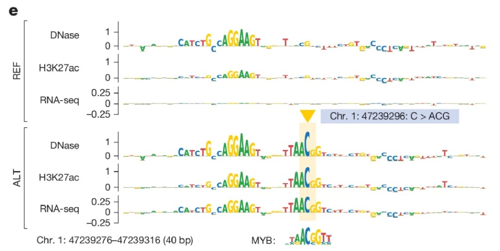
Fig 6e: ISM MYB motif logos
Two inserted letters → new MYB binding motif → MYB binds → chromatin opens → enhancer activated → TAL1 expressed → T-cell proliferation → T-ALL
This is not a cherry-picked example. The paper's enrichment analysis shows that 50% of Mendelian disease variants produce effects in both local chromatin regulation and gene expression simultaneously, with 8x enrichment over matched control variants. Most disease non-coding variants have multimodal consequences. Models that look at only one modality are structurally incomplete for variant interpretation.
Benchmarks: What the Numbers Tell You
A few key numbers worth internalizing before you run your own analyses.
On variant effect prediction, AlphaGenome matches or exceeds the best available specialist model on 25 of 26 benchmarks, including beating ChromBPNet on chromatin accessibility, Pangolin and SpliceAI on splicing and Orca on contact maps.
eQTL direction prediction accuracy runs 70–75% auROC across most GTEx tissues. This sounds moderate until you appreciate the task: predicting, from sequence alone, the direction of a statistical association measured across hundreds of people, with linkage disequilibrium and measurement noise on top of the actual molecular effect. The signed correlation between predicted effect sizes and observed GTEx effects is 0.39–0.50, the authors are honest that this reflects the genuine difficulty of the problem.
The most clinically relevant benchmark is GWAS coverage. The current gold standard, eQTL colocalization using GTEx, resolves around 15% of disease-associated loci. AlphaGenome, at an 80% directional accuracy threshold, resolves approximately 40%. Two to three times more GWAS loci, specifically because the model predicts from sequence rather than requiring the variant to have been measured experimentally in the right tissue.
Practical Gotchas Before You Run It
Window centering. The model scores a variant using a 1 Mb window centered on that position. Variants near the window edge have asymmetric context. The API centers automatically for standard variant scoring, but be aware of this for custom queries, mis-centering can meaningfully degrade predictions for variants with known distant regulatory interactions.
Reference genome. The model was trained on hg38 for human and mm10 for mouse. If your coordinates are in hg19/GRCh37, liftover first. This is the most common source of silently wrong results.
Cell type availability. The model predicts well for the major GTEx tissues and ENCODE cell lines. For rare cell types or understudied tissues, predictions are less reliable, the model extrapolates from the nearest related cell type it was trained on.
What the model cannot do. AlphaGenome predicts relative changes, not absolute values. It tells you a variant reduces RNA-seq signal in liver, not what the absolute expression level is. It scores one variant at a time against the reference genome, so combinatorial effects of multiple variants in the same regulatory region aren't captured. And it doesn't incorporate evolutionary conservation, protein structural effects, or population genetics data, integrating those external signals is something you'd build on top.
Running It
For most use cases, the AlphaGenome API is the right starting point, free for non-commercial use, handles the distilled model, window centering and reverse complement averaging automatically.
For custom data, fine-tuning on novel cell types, or integrating AlphaGenome into a PyTorch pipeline, the Kundaje Lab at Stanford released a faithful PyTorch port in early 2026. Numerically equivalent to the JAX original, GPU-compatible without TPUs, available via:
pip install alphagenome-pytorchPart 3 puts this into practice. We'll run a saturation mutagenesis analysis, mutating every position across a disease-relevant enhancer, scoring each mutation across all output heads and building a base-resolution regulatory impact map. The kind of analysis directly relevant to base editing therapeutic design. On a MacBook, using the API.
Citation
Avsec Ž, et al. Advancing regulatory variant effect prediction with AlphaGenome. Nature. 2026. Published 28 January 2026. https://doi.org/10.1038/s41586-025-10014-0