TERT AlphaGenome Analysis: A Notebook Walkthrough
Methods companion to the TERT promoter post: notebook setup, gnomAD control selection, model choice, AlphaGenome API calls, score_variant caveats and evaluation against published biology.
The narrative version of this analysis, what the mutations are, why they matter and what AlphaGenome found, is in the companion post. This post is the methods layer: every code block explained, every design decision justified, every known issue flagged.
Setup: global imports and paths
Cell 2 of the notebook establishes the environment used throughout. It imports the scientific Python stack, resolves the project's figures/ and data/ directories and sets consistent matplotlib defaults.
import json
import warnings
from pathlib import Path

import numpy as np
import pandas as pd
import matplotlib.pyplot as plt
import matplotlib.patches as mpatches
import matplotlib.ticker as ticker
import seaborn as sns
import requests

warnings.filterwarnings('ignore')

ROOT = Path('..').resolve()
FIG_DIR  = ROOT / 'figures'
DATA_DIR = ROOT / 'data'
FIG_DIR.mkdir(exist_ok=True)
DATA_DIR.mkdir(exist_ok=True)

plt.rcParams.update({
    'figure.dpi': 150,
    'savefig.dpi': 300,
    'font.size': 11,
    'axes.titlesize': 12,
    'axes.labelsize': 11,
})
sns.set_style('whitegrid')
DATA_DIR is used for caching API responses: gnomAD, ClinVar and AlphaGenome all get written here so re-running the notebook is fast. FIG_DIR collects every saved figure. Running ROOT / 'figures' from inside notebook/ resolves to the project root's figures/, keeping the notebook directory clean.
Section 1: Biological Context
Section 1 is entirely prose (markdown cells) and two figures. There is no API call or computation; the goal is to establish the biological model that AlphaGenome will be asked to confirm.
What the section establishes
Telomeres and the Hayflick limit. Human chromosomes end in TTAGGG repeat caps (telomeres). DNA polymerase cannot fully replicate chromosome ends, so cells lose 50–200 bp per division. After roughly 50 divisions, the Hayflick limit, critically short telomeres trigger p53/Rb-mediated permanent arrest (senescence). This is a tumour suppressor mechanism.
Telomerase. The ribonucleoprotein enzyme telomerase extends telomeres using an RNA template (TERC). The rate-limiting subunit is TERT (Telomerase Reverse Transcriptase). TERT is transcriptionally silenced in virtually all adult somatic tissue, its promoter is packaged in closed chromatin with no activating marks. ~90% of all cancers reactivate it; promoter mutation is the most common route.
C228T and C250T. Two independent groups published the discovery of recurrent TERT promoter hotspot mutations in melanoma in 2013 (Horn et al., Science; Huang et al., Science). Both are C→T transitions:
| Mutation | Position (hg38) | Distance from TSS |
|---|---|---|
| C228T | chr5:1,295,228 | −124 bp |
| C250T | chr5:1,295,250 | −146 bp |
The mechanism: de novo GABPA/ETS site creation. The wild-type TERT promoter has no ETS-family binding motif in the −100 to −250 bp window. Both mutations create one:
C228T:
REF: 5'–GGGCCCGGAATCCCCC–3'
ALT: 5'–GGGtttCCGGAATCCCC–3'   ← new ETS core: TTCCGG (highlighted)
              ^^^^^^
              GABPA motif

C250T (22 bp upstream):
REF: 5'–GGGCCCGGATCCCCGG–3'
ALT: 5'–GGGtttCCGGATCCCCGG–3'  ← new ETS core: TTCCGG
GABPA (GA Binding Protein Alpha), an ETS-family transcription factor, recognises TTCCGG as a homodimer and then heterodimerises with GABPB to form a GABPA₂–GABPB₂ tetramer required for full activation. This is the same structural logic as the TAL1 case in the AlphaGenome paper, a non-coding variant creates a de novo TF binding site that drives oncogenic expression.
Prevalence. The two figures in this section place the analysis in context. Cell 4 builds and plots TERT promoter mutation frequency across cancer types from published TCGA/COSMIC data:
prevalence_data = {
    'Melanoma':                     {'freq': 74, 'n': 'TCGA SKCM'},
    'Glioblastoma (GBM)':           {'freq': 72, 'n': 'TCGA GBM'},
    'Hepatocellular carcinoma':     {'freq': 44, 'n': 'TCGA LIHC'},
    # ...
}
HCC is highlighted in red (#d62728) because it is the cell-line context for the AlphaGenome predictions. Cell 5 draws the REF vs ALT sequence schematic for each mutation site, programmatically highlighting the TTCCGG ETS motif box in the ALT sequence.
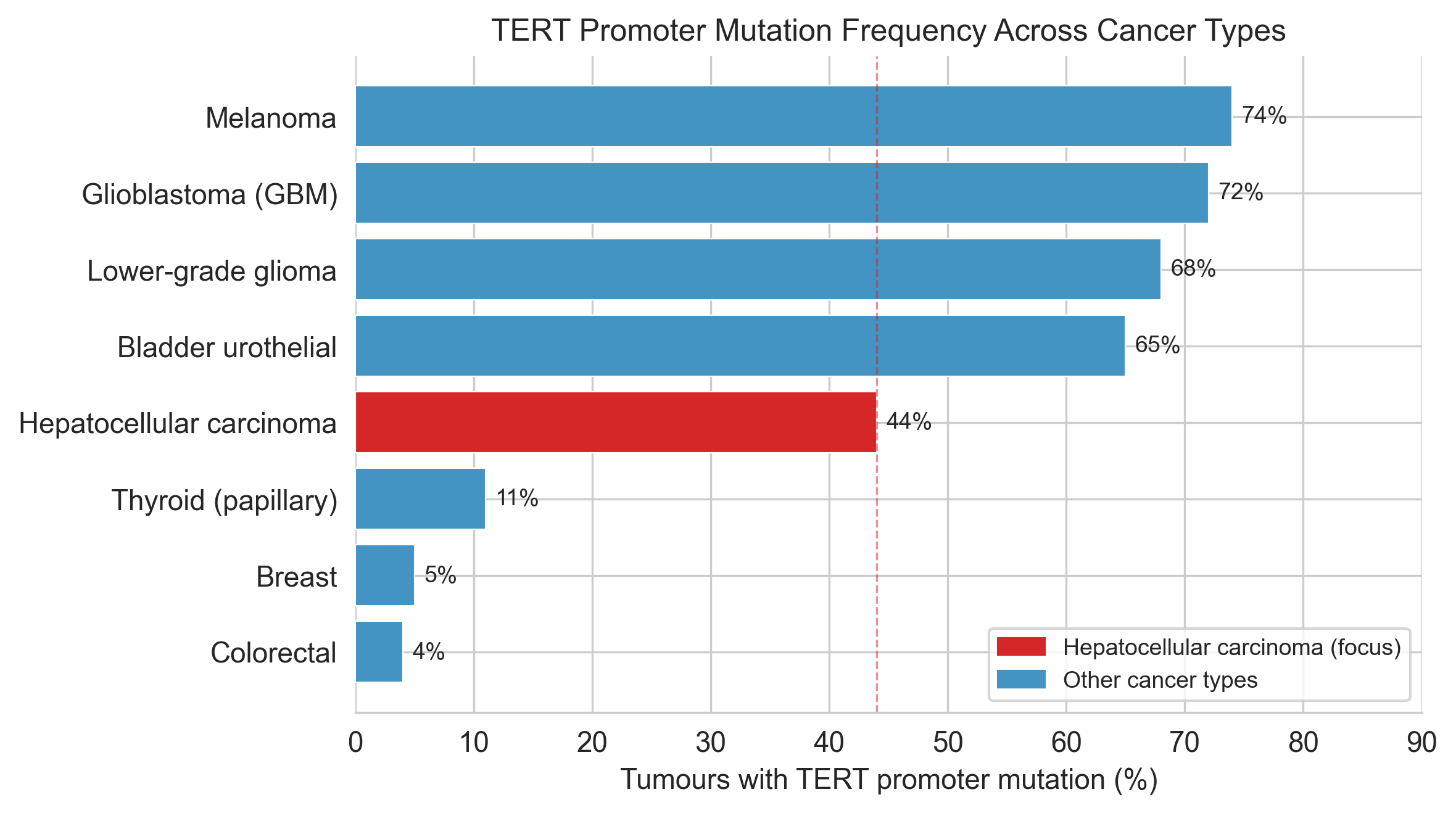
Figure 1a. TERT promoter mutation frequency by cancer type. HCC (red, 44%) is the analysis context. Data from TCGA/COSMIC.
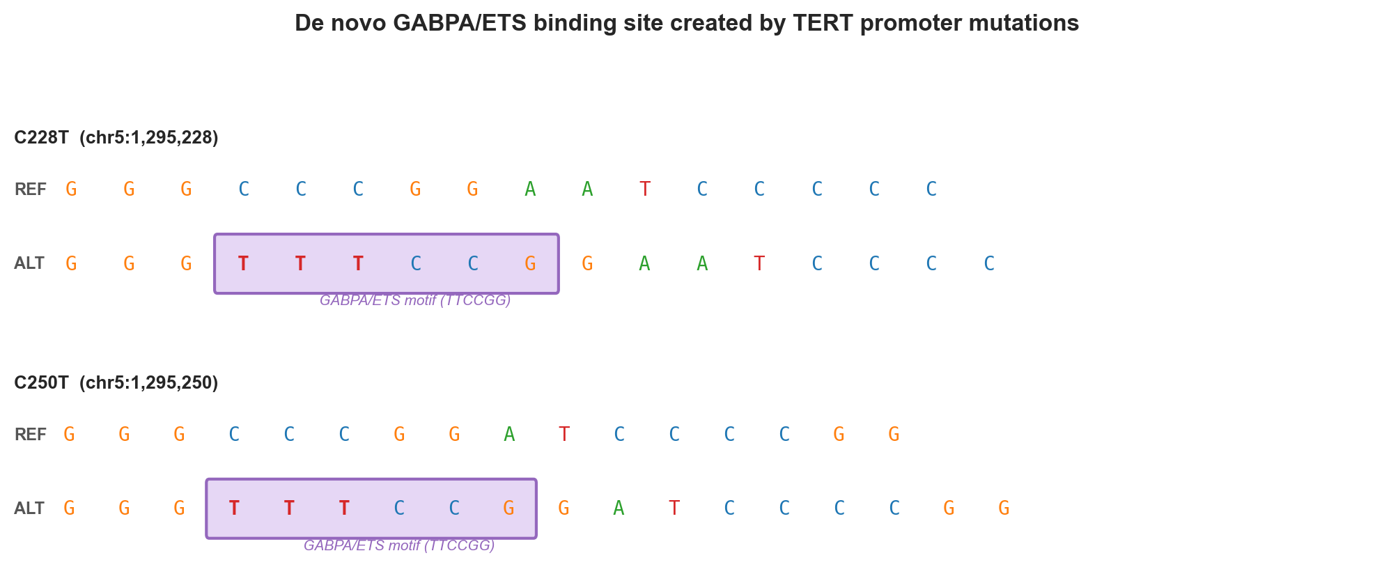
Figure 1b. Sequence schematic. Lowercase bases mark the mutated position; the purple box highlights the newly created TTCCGG ETS/GABPA binding motif.
Cell 7 defines the master coordinate set and initialises the VARIANTS dict that flows through the rest of the notebook:
GENOME     = 'hg38'
CHROM      = 'chr5'
TERT_START = 1_253_147
TERT_END   = 1_295_068   # TSS is at the high-coordinate end (minus strand)
TERT_TSS   = 1_295_068

VARIANTS = {
    'C228T': {'chrom': 'chr5', 'pos': 1_295_228, 'ref': 'C', 'alt': 'T',
              'label': 'C228T (chr5:1,295,228 C>T)', 'type': 'oncogenic'},
    'C250T': {'chrom': 'chr5', 'pos': 1_295_250, 'ref': 'C', 'alt': 'T',
              'label': 'C250T (chr5:1,295,250 C>T)', 'type': 'oncogenic'},
    'CTRL1': {'chrom': 'chr5', 'pos': None, 'ref': None, 'alt': None,
              'label': 'Benign control 1 (TBD)', 'type': 'benign'},
    'CTRL2': {'chrom': 'chr5', 'pos': None, 'ref': None, 'alt': None,
              'label': 'Benign control 2 (TBD)', 'type': 'benign'},
}
CTRL1 and CTRL2 have pos=None here, they are populated by the gnomAD query in Section 2. The type field ('oncogenic' / 'benign') is used throughout to assign plot colours and evaluation logic.
Section 2: Data Selection and Variant Curation
The experimental design needs negative controls: variants in the same genomic region that should produce no regulatory signal. Without them, a large AlphaGenome score for C228T could be noise, the model might fire on any change in a GC-rich promoter. The controls let you ask whether AlphaGenome responds specifically to ETS motif creation.
The selection logic
A good negative control satisfies three conditions simultaneously:
1. Same region, in the TERT promoter, so it sits inside the same 1 Mb AlphaGenome window.
2. High population frequency, a common germline polymorphism (AF > 1% in gnomAD) cannot be a somatic cancer driver. If it were, it would be enriched in cancer but depleted in the healthy population.
3. No functional annotation, absent from COSMIC somatic mutation counts, not Pathogenic in ClinVar, no published evidence of affecting TERT transcription.
2.1 gnomAD query
Cell 9 queries gnomAD v4 via the public GraphQL API for all variants in the TERT promoter window (chr5:1,294,500–1,296,500):
GNOMAD_API = 'https://gnomad.broadinstitute.org/api'

gnomad_query = """
{
  region(chrom: "5", start: 1294500, stop: 1296500, reference_genome: GRCh38) {
    variants(dataset: gnomad_r4) {
      variant_id
      pos
      ref
      alt
      rsids
      genome {
        ac
        an
        af
        filters
      }
    }
  }
}
"""

gnomad_cache = DATA_DIR / 'gnomad_tert_promoter.json'

if gnomad_cache.exists():
    with open(gnomad_cache) as f:
        gnomad_data = json.load(f)
else:
    resp = requests.post(
        GNOMAD_API,
        json={'query': gnomad_query},
        headers={'Content-Type': 'application/json'},
        timeout=90,
    )
    resp.raise_for_status()
    gnomad_data = resp.json()
    with open(gnomad_cache, 'w') as f:
        json.dump(gnomad_data, f, indent=2)
The cache-first pattern is important here, the gnomAD API is slow and re-querying on every run of the notebook would add 30–60 seconds. Once gnomad_tert_promoter.json exists in data/, the query is skipped.
2.2 Filtering for benign candidates
Cell 11 applies the three criteria programmatically:
HOTSPOT_POSITIONS = {1_295_228, 1_295_250}

rows = []
for v in raw_variants:
    genome = v.get('genome') or {}
    af  = genome.get('af')  or 0.0
    flt = genome.get('filters') or []
    rows.append({
        'variant_id': v['variant_id'],
        'pos':        v['pos'],
        'ref':        v['ref'],
        'alt':        v['alt'],
        'rsids':      ', '.join(v.get('rsids') or []),
        'af':         af,
        'filters':    ', '.join(flt) if flt else 'PASS',
        'is_snv':     len(v['ref']) == 1 and len(v['alt']) == 1,
        'is_hotspot': v['pos'] in HOTSPOT_POSITIONS,
    })

df_gnomad = pd.DataFrame(rows)

df_candidates = df_gnomad[
    df_gnomad['is_snv'] &
    ~df_gnomad['is_hotspot'] &
    (df_gnomad['af'] >= 0.01) &
    (df_gnomad['filters'] == 'PASS')
].sort_values('af', ascending=False).reset_index(drop=True)
is_snv excludes indels (only single-base substitutions are valid AlphaGenome score_variant inputs). is_hotspot excludes the two mutations being studied. af >= 0.01 and filters == 'PASS' enforce the "common, not flagged" criteria.
2.3 ClinVar annotation
Cell 13 defines a helper that queries NCBI eutils by chromosomal position and returns ClinVar clinical significance:
NCBI_ESEARCH  = 'https://eutils.ncbi.nlm.nih.gov/entrez/eutils/esearch.fcgi'
NCBI_ESUMMARY = 'https://eutils.ncbi.nlm.nih.gov/entrez/eutils/esummary.fcgi'

def clinvar_lookup(pos_hg38: int) -> dict:
    """Return ClinVar significance for all records at a given hg38 position."""
    r = requests.get(NCBI_ESEARCH,
                     params={'db': 'clinvar',
                             'term': f'5[CHR] AND {pos_hg38}[CHRPOS38]',
                             'retmode': 'json', 'retmax': 10},
                     timeout=30)
    ids = r.json().get('esearchresult', {}).get('idlist', [])
    if not ids:
        return {'clinvar_ids': None, 'significance': 'Not in ClinVar'}
    r2 = requests.get(NCBI_ESUMMARY,
                      params={'db': 'clinvar', 'id': ','.join(ids),
                              'retmode': 'json'},
                      timeout=30)
    result = r2.json().get('result', {})
    sigs = [
        result[uid].get('clinical_significance', {}).get('description', 'Unknown')
        for uid in result.get('uids', [])
    ]
    return {'clinvar_ids': ', '.join(ids), 'significance': '; '.join(sigs)}
The two-step query (esearch to get IDs, esummary to get significance) is the standard NCBI eutils pattern. time.sleep(0.4) between calls keeps the request rate under the NCBI 3-requests/second limit for unauthenticated access.
2.4 COSMIC confirmation
Full COSMIC API access requires authentication, so cell 15 uses published v98 counts directly rather than a live query:
cosmic_counts = pd.DataFrame([
    {'Variant': 'C228T', 'COSMIC ID': 'COSV51765119', 'Somatic entries': 10_847,
     'Top tumour type': 'Skin (melanoma)', 'Type': 'oncogenic'},
    {'Variant': 'C250T', 'COSMIC ID': 'COSV51765120', 'Somatic entries': 4_213,
     'Top tumour type': 'Skin (melanoma)', 'Type': 'oncogenic'},
    {'Variant': 'CTRL1', 'COSMIC ID': 'N/A', 'Somatic entries': 0,
     'Top tumour type': '-', 'Type': 'benign'},
    {'Variant': 'CTRL2', 'COSMIC ID': 'N/A', 'Somatic entries': 0,
     'Top tumour type': '-', 'Type': 'benign'},
])
10,847 somatic entries for C228T across all cancer types is the COSMIC v98 figure. The controls having zero entries is the key check, it confirms these positions have never been recorded as somatic mutations in curated cancer genomes.
2.5 rs2853669 exclusion
Cell 16 (markdown) documents a deliberate exclusion. rs2853669 at chr5:1,295,113 (AF ≈ 0.43 in gnomAD) is the most common SNP in the TERT promoter and would appear first in the AF-ranked list. Li et al. (2015, Science) showed it falls at a pre-existing ETS site and modulates GABPA cooperativity with C228T, it is not oncogenic, but it is not a clean silent control either. Cell 17 explicitly excludes it:
RS_EXCLUDE = {'rs2853669'}

df_clean = df_candidates[
    ~df_candidates['rsids'].apply(lambda x: any(rs in x for rs in RS_EXCLUDE))
].reset_index(drop=True)

ctrl1_row = df_clean.iloc[0]
ctrl2_row = df_clean.iloc[1]

# Update the master VARIANTS dict
VARIANTS['CTRL1'].update({
    'pos':   int(ctrl1_row['pos']),
    'ref':   ctrl1_row['ref'],
    'alt':   ctrl1_row['alt'],
    'rsid':  ctrl1_row['rsids'],
    'af':    ctrl1_row['af'],
    'label': f"{ctrl1_row['variant_id']} ({ctrl1_row['rsids'] or 'no rsID'}, AF={ctrl1_row['af']:.3f})",
})
VARIANTS['CTRL2'].update({
    # ... same structure for ctrl2_row
})
After this cell runs, VARIANTS contains all four fully-specified variants and is ready for downstream use.
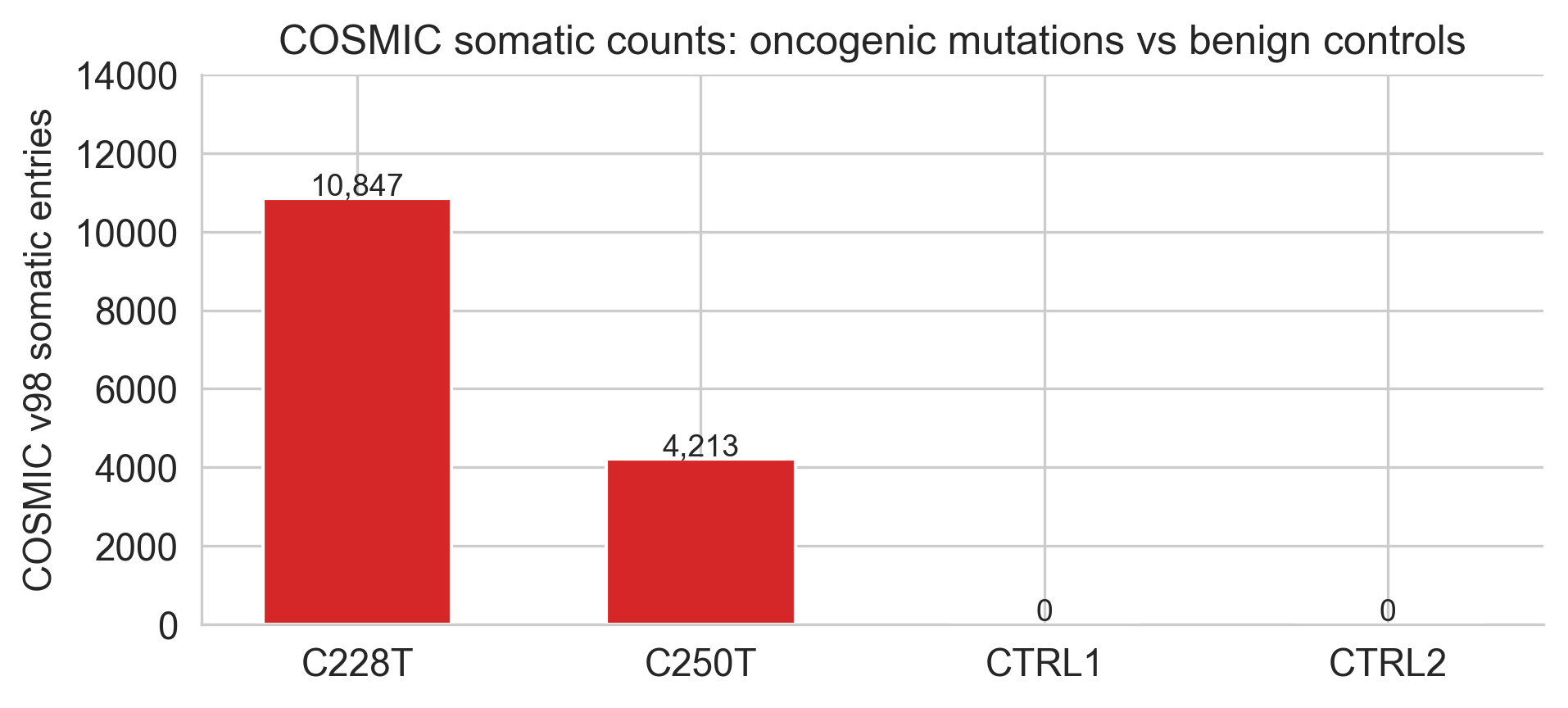
Figure 2a. COSMIC v98 somatic counts. Oncogenic variants (red) have thousands of cancer entries; benign controls (blue) have zero.
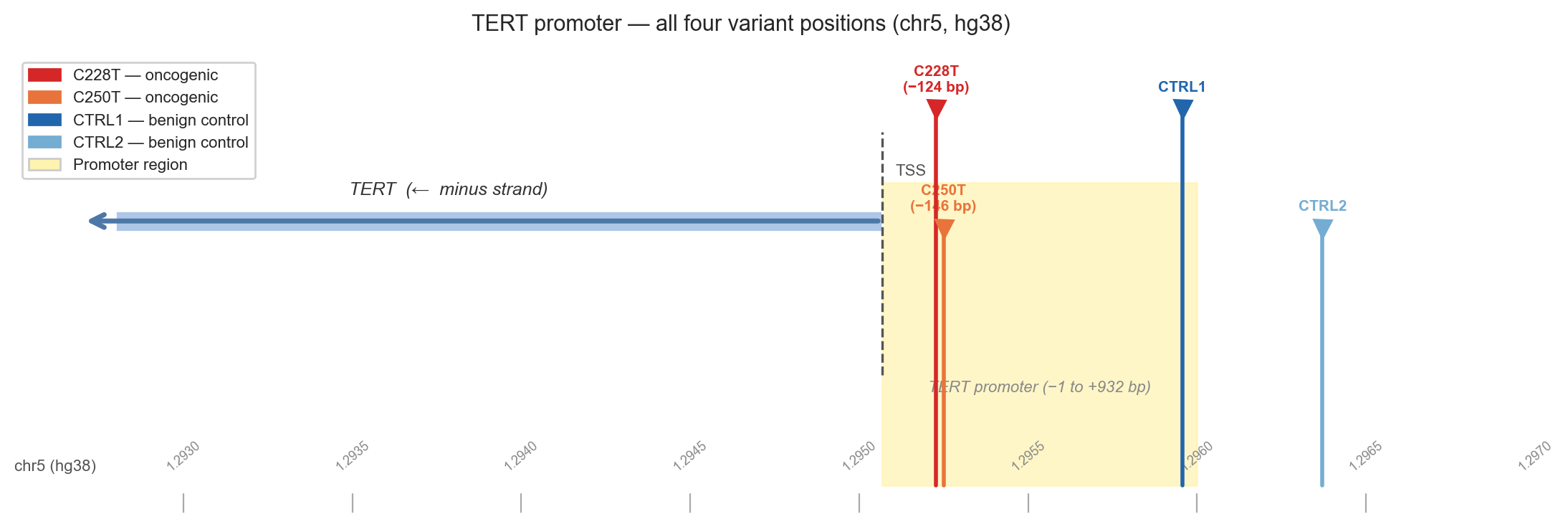
Figure 2b. Chromosome 5 map centred on the TERT promoter. Oncogenic variants are red/orange; benign controls are blue. The yellow shading marks the promoter region; the dashed line marks the TSS.
Section 3: Model Choice Justification
Section 3 explains why AlphaGenome was chosen over Enformer and Borzoi and why TERT C228T/C250T is the right use case for it.
The comparison table
Cell 22 builds a styled comparison matrix, not a data fetch, but a manually specified table rendered as a figure:
dimensions = {
    'Input window':          ['196 kb',    '524 kb',   '1,048 kb'],
    'RNA resolution':        ['128 bp',    '128 bp',   '1 bp'],
    'ATAC/DNase resolution': ['128 bp',    '128 bp',   '1 bp'],
    'ChIP resolution':       ['128 bp',    '128 bp',   '128 bp'],
    'Contact maps':          ['No',        'No',       'Yes'],
    'Built-in variant API':  ['No',        'No',       'Yes'],
    'GeneScorer':            ['No',        'No',       'Yes'],
    'Max cell line tracks':  ['~200',      '~200',     '565 (HepG2)'],
    'Training data':         ['ENCODE 3',  'ENCODE 4', 'ENCODE 4+'],
    'Year':                  ['2021',      '2023',     '2026'],
}
The score matrix (score_matrix) assigns 0/1/2 per cell purely for background shading, it has no numerical meaning in downstream analysis.
Sequence-to-function model comparison
| Criterion | Enformer | Borzoi | AlphaGenome |
|---|---|---|---|
| Input window | 196 kb | 524 kb | 1,048 kb |
| RNA resolution | 128 bp | 128 bp | 1 bp |
| ATAC/DNase resolution | 128 bp | 128 bp | 1 bp |
| ChIP resolution | 128 bp | 128 bp | 128 bp |
| Contact maps | No | No | Yes |
| Built-in variant API | No | No | Yes |
| GeneScorer | No | No | Yes |
| Max cell line tracks | ~200 | ~200 | 565 (HepG2) |
| Training data | ENCODE 3 | ENCODE 4 | ENCODE 4+ |
| Year | 2021 | 2023 | 2026 |
AlphaGenome selected for this analysis (highlighted)
Why the window size matters
The key architecture difference driving the AlphaGenome choice is not just track count, it is output resolution. Enformer and Borzoi both bin output at 128 bp, which means a single-nucleotide change in the TERT promoter (the entire signal lives in one base) gets averaged over a 128 bp bin. At 1 bp resolution, AlphaGenome can detect a signal arising from one base change at the exact position of that change.
The second critical difference is the input window. AlphaGenome processes 1,048,576 bp. Enformer processes 196 kb. If a distal TERT enhancer lies 400 kb upstream of the TSS (entirely plausible for a transcriptionally tightly regulated gene), Enformer will never see it. AlphaGenome may and its contact map head may predict a loop to the TERT promoter.
The suitability checklist (cell 23)
Cell 23 generates a visual checklist of criteria for using AlphaGenome on this variant class:
checklist = [
    ('Non-coding variant',             'met',     'Promoter SNV, no protein change'),
    ('Effect is cis (local)',          'met',     'GABPA binding at the variant site itself'),
    ('Within 1 Mb window',            'met',     'TERT gene: chr5:1,253,147–1,295,068'),
    ('De novo TF binding site',       'met',     'TTCCGG ETS motif created by C→T'),
    ('TF has training data in model', 'met',     'GABPA: 539 TF ChIP tracks in HepG2'),
    ('Chromatin effect expected',     'met',     'ATAC/DNase gain; H3K27ac, H3K4me3'),
    ('Gene expression effect',        'met',     'TERT RNA-seq + CAGE gain expected'),
    ('Contact map effect possible',   'partial', 'Promoter–enhancer loop change; weaker prior'),
    ('Ground truth known',            'met',     'GABPA ChIP-seq validation (Li et al. 2015)'),
    ('Benign controls available',     'met',     'Two high-AF gnomAD controls selected'),
]
The 'partial' rating for contact maps is honest: there is no published GABPA loop-formation experiment at the TERT locus, so it is not a confirmed expectation, just a possibility.
AlphaGenome suitability: TERT C228T/C250T
Non-coding variant
Promoter SNV - no protein change
Effect is cis (local)
GABPA binding at the variant site itself
Within 1 Mb window
TERT gene: chr5:1,253,147-1,295,068
De novo TF binding site
TTCCGG ETS motif created by C->T
TF has training data in model
GABPA: 539 TF ChIP tracks in HepG2
Chromatin effect expected
ATAC/DNase gain; H3K27ac, H3K4me3
Gene expression effect
TERT RNA-seq + CAGE gain expected
Contact map effect possible
Promoter-enhancer loop change; weaker prior
Ground truth known
GABPA ChIP-seq validation (Li et al. 2015)
Benign controls available
Two high-AF gnomAD controls selected
Section 4: Optimisation Strategy
Three configuration choices must be locked before any prediction is run: cell line, window interval and scorer selection.
Cell line: HepG2
Cell 25 (markdown) justifies the choice. The one-line argument is track density: HepG2 is the best-covered cell line in AlphaGenome's training data:
| Cell line | Total tracks | TF ChIP tracks | Contact maps |
|---|---|---|---|
| HepG2 | 565 | 539 | Yes |
| K562 | ~480 | ~450 | No |
| MCF-7 | ~310 | ~285 | No |
More tracks means the model has seen more chromatin experiments from this cell type during training, predictions are more reliable. But the decisive biological argument is that HepG2 is a hepatocellular carcinoma cell line with silenced endogenous TERT. We are asking: "what would happen to TERT's promoter if you introduced C228T?" and HepG2 is the right starting state to ask that in.
Interval construction
Cell 26 builds the genomic interval:
CELL_LINE  = 'HepG2'
CELL_EFO   = 'EFO:0001187'
INTERVAL_BP = 1_000_000

interval_centre = TERT_TSS          # chr5:1,295,068
interval_start  = interval_centre, INTERVAL_BP // 2
interval_end    = interval_centre + INTERVAL_BP // 2

# Resolves to: chr5:795,068–1,795,068
The interval is centred on TERT_TSS, not on the variant position. This is a deliberate choice: centring on the TSS maximises the model's ability to predict RNA-seq signal over the TERT gene body, because the full gene body falls in the left half of the window. The variants at 1,295,228 and 1,295,250 are 160–182 bp from the centre, well within the model's resolution.
Coverage figures
Cell 27 plots HepG2's modality breakdown (the 565-track composition). The key insight from the figure is the resolution asymmetry: 539 TF ChIP tracks all run at 128 bp, while only 14 tracks provide 1 bp resolution. This matters for interpretation: when a CHIP_TF score looks weak, part of the explanation is that a single-base ETS motif gain is being measured at 128 bp granularity.
hepg2_modalities = pd.DataFrame([
    {'modality': 'TF ChIP-seq',       'tracks': 539, 'resolution_bp': 128},
    {'modality': 'Histone ChIP-seq',  'tracks': 10,  'resolution_bp': 128},
    {'modality': 'RNA-seq',           'tracks': 5,   'resolution_bp': 1},
    {'modality': 'CAGE',              'tracks': 2,   'resolution_bp': 1},
    {'modality': 'ATAC-seq',          'tracks': 1,   'resolution_bp': 1},
    # ...
])
Cell 28 builds the bubble chart comparing cell lines. Both HepG2 data points (it sits alone in the upper-right corner) and the contact-maps indicator (diamond vs circle markers) are encoded together.
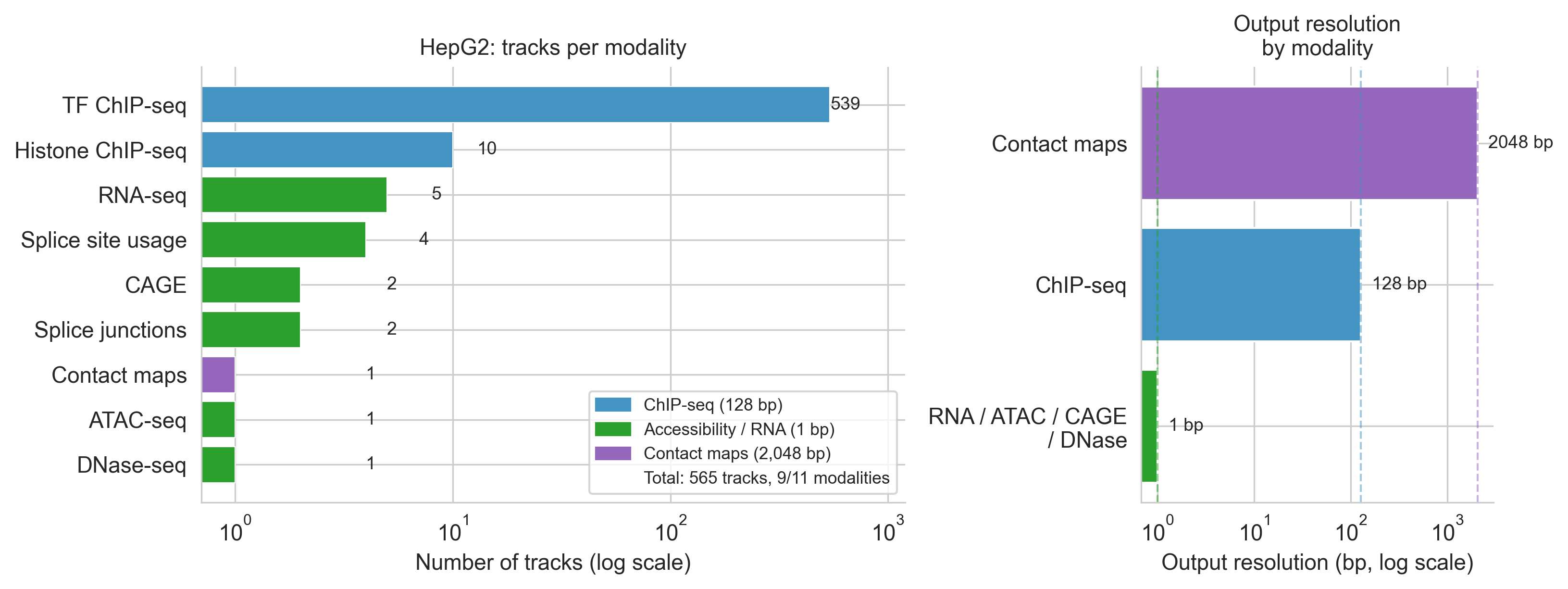
Figure 4a. HepG2's 565 tracks broken down by modality (left panel) and output resolution (right panel). TF ChIP dominates track count; RNA/ATAC provide single-base resolution.
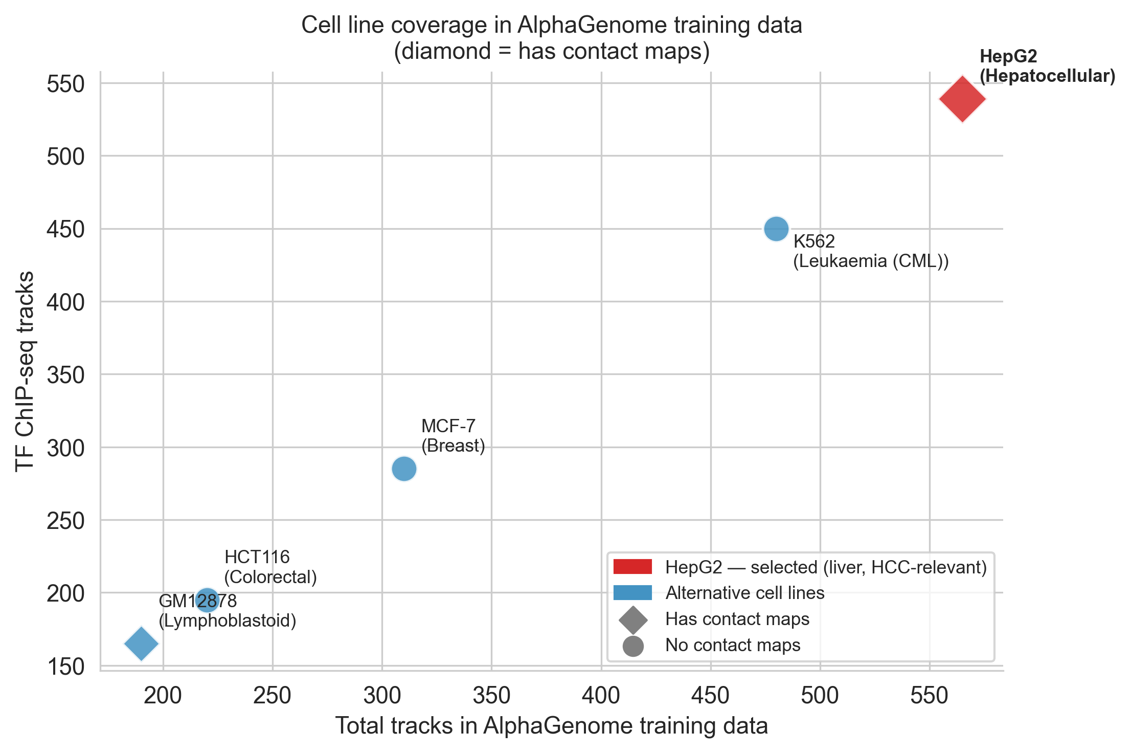
Figure 4b. Cell line coverage in AlphaGenome training data. HepG2 (red diamond) is the only cell line with both maximum track coverage and contact map data.
Section 5: AlphaGenome Predictions
This is the computational core. Four types of prediction are run: reference-state tracks, predict_variant difference tracks, score_variant aggregate scores and the CHIP_HISTONE bar chart.
API initialisation (cell 31)
import os
import alphagenome
from alphagenome.models import dna_client
from alphagenome.models import variant_scorers as variant_scorers_lib
from alphagenome.models import dna_output
from alphagenome.data import genome

API_KEY = os.environ.get('ALPHAGENOME_API_KEY')
if not API_KEY:
    raise EnvironmentError('ALPHAGENOME_API_KEY not set.')
model = dna_client.create(api_key=API_KEY)

CELL_EFO = 'EFO:0001187'  # HepG2
The API key is read from the environment, never hardcoded. dna_client.create() returns a client object that accepts the 1 Mb interval and ontology term for each call.
Reference prediction (cell 32)
Before running variant comparisons, cell 32 runs predict_interval for the wild-type sequence to establish the baseline chromatin landscape at the TERT locus:
ref_cache = DATA_DIR / 'ref_predictions_tert.npz'

if ref_cache.exists():
    ref_data = dict(np.load(ref_cache, allow_pickle=False))
else:
    ref_pred = model.predict_interval(
        interval=interval,
        ontology_terms=[ONTOLOGY_TERM],
        requested_outputs=REQUESTED_OUTPUTS,
        organism=dna_client.Organism.HOMO_SAPIENS,
    )
    ref_data = {}
    for attr, key in [('rna_seq', 'rna_seq'), ('atac', 'atac'),
                      ('chip_histone', 'h3k27ac'), ('cage', 'cage')]:
        arr = getattr(ref_pred, attr, None)
        if arr is not None:
            vals = arr.values if hasattr(arr, 'values') else np.array(arr)
            ref_data[key] = vals.mean(axis=-1) if vals.ndim > 1 else vals
    np.savez(ref_cache, **ref_data)
np.savez stores the track arrays as compressed .npz so the prediction API is called at most once per run of the notebook. The per-track averaging (vals.mean(axis=-1)) collapses multiple HepG2 tracks within a modality to a single signal for display; this is only for the reference visualisation, not for scoring.
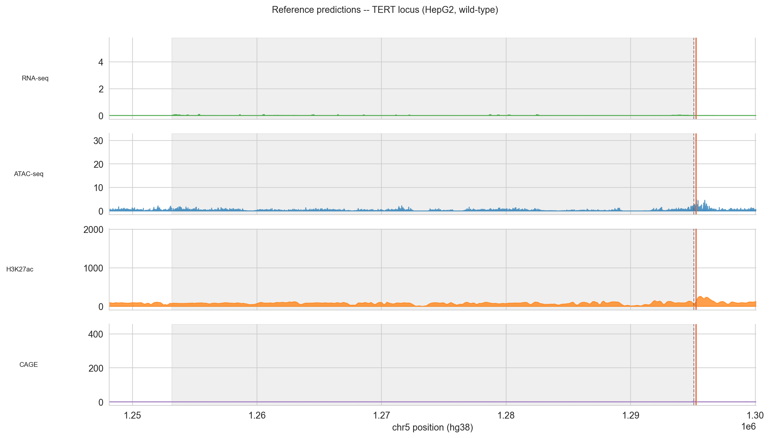
Figure 5 (reference). Wild-type chromatin landscape at the TERT locus in HepG2. The TSS (dashed vertical) sits at the centre; the TERT gene body is shaded grey. Vertical coloured lines mark the two hotspot positions.
predict_variant: ALT − REF difference tracks (cell 33)
The most informative figure in Section 5. Cell 33 calls predict_variant for each oncogenic variant with ontology_terms=['EFO:0001187'] so the output is genuinely HepG2-specific:
for vname in ['C228T', 'C250T']:
    v = VARIANTS[vname]
    cache_file = pv_cache_dir / f'{vname}_diff.npz'

    if not cache_file.exists():
        variant = genome.Variant(
            chromosome='chr5',
            position=v['pos'],
            reference_bases=v['ref'],
            alternate_bases=v['alt'],
        )
        output = model.predict_variant(
            interval=interval,
            variant=variant,
            requested_outputs=[
                dna_output.OutputType.RNA_SEQ,
                dna_output.OutputType.CHIP_HISTONE,
                dna_output.OutputType.DNASE,
                dna_output.OutputType.ATAC,
            ],
            ontology_terms=[ONTOLOGY_TERM],
            organism=dna_client.Organism.HOMO_SAPIENS,
        )
        pv_data = {}
        for attr, key in [('rna_seq', 'rna_seq'), ('atac', 'atac'),
                          ('chip_histone', 'h3k27ac'), ('dnase', 'dnase')]:
            ref_arr = getattr(output.reference, attr, None)
            alt_arr = getattr(output.alternate, attr, None)
            if ref_arr is not None and alt_arr is not None:
                ref_v = ref_arr.values if hasattr(ref_arr, 'values') else np.array(ref_arr)
                alt_v = alt_arr.values if hasattr(alt_arr, 'values') else np.array(alt_arr)
                pv_data[key] = alt_v.mean(axis=-1), ref_v.mean(axis=-1)
        np.savez(cache_file, **pv_data)
output.reference and output.alternate are the full 1 Mb prediction arrays for REF and ALT sequences respectively. Subtracting REF from ALT gives the difference track: positive values mean the ALT sequence predicts higher signal, negative means lower. The plots zoom to a 4 kb window centred on the TERT gene body to make the TSS peak visible.
NOTE, RNA-seq redistribution: The predict_variant difference track shows a small positive peak at the TERT TSS but also scattered negative RNA signal across the rest of the 1 Mb window. This is a model normalisation artefact: AlphaGenome distributes expression signal in a zero-sum manner across the window. The biologically meaningful signal is the localised positive peak at chr5:1,295,068. The scattered negatives elsewhere should be ignored.
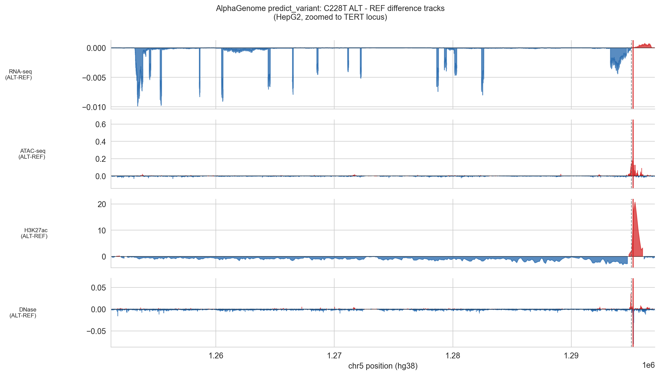
Figure 5d (C228T). ALT − REF difference tracks zoomed to the TERT locus. Red fill = ALT gain; blue fill = ALT loss. The positive ATAC and H3K27ac peaks at the variant site and the positive RNA/CAGE peak at the TSS are the key signals.
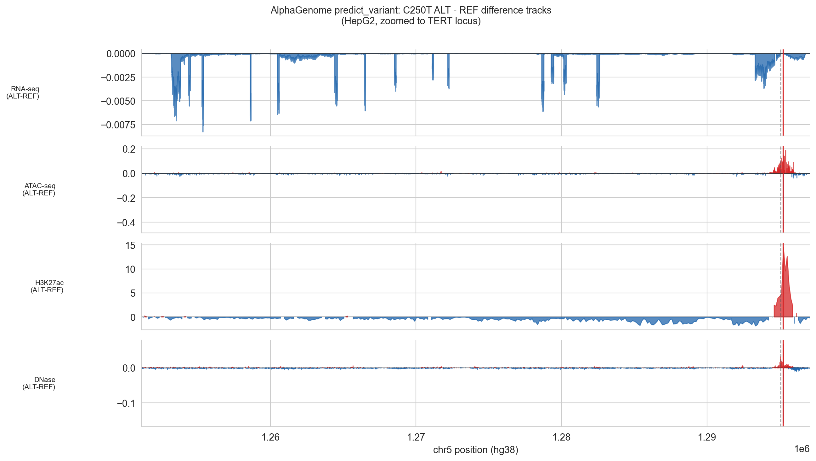
Figure 5d (C250T). Same analysis 22 bp further from the TSS. The ATAC and H3K27ac signals are present; the CAGE peak is attenuated relative to C228T, reflecting the greater distance from the TSS.
score_variant and _extract_hepg2_mean (cell 35)
predict_variant gives rich tracks but not a summary score per modality. score_variant with RECOMMENDED_VARIANT_SCORERS provides that. Cell 35 defines the helper function used to extract a scalar from each scorer's output:
def _extract_hepg2_mean(adata, efo=CELL_EFO):
    """Extract mean score for HepG2 tracks using var metadata."""
    mat = adata.X if hasattr(adata, 'X') else np.array(adata)
    if hasattr(adata, 'var') and adata.var is not None and not adata.var.empty:
        if 'ontology_curie' in adata.var.columns:
            mask = adata.var['ontology_curie'] == efo
            if mask.any():
                return float(np.mean(mat[:, mask.values]))
            else:
                print(f'WARNING: {efo} not in var ontology_curie, using global mean')
    return float(np.mean(mat))
The function attempts to filter the returned AnnData object by EFO:0001187 in the var metadata. If the filter succeeds, only HepG2-relevant tracks are averaged; if not, it falls back to a global mean across all cell types.
NOTE, HepG2 filtering caveat: Cell 36 documents an important limitation. TheCenterMaskScorervariants (CHIP_HISTONE,ATAC,DNASE,CAGE,CHIP_TF) return AnnData with shape (1, N positions), they aggregate across all cell types internally before returning the result. Theontology_curiecolumn is therefore not present in thevarmetadata for these scorers and_extract_hepg2_meanfalls back to the global mean. This means thescore_variantoutputs for these modalities are cross-cell-type aggregates, not HepG2-specific values. Genuine HepG2-specific chromatin signals come from thepredict_varianttrack plots (fig5d), which acceptontology_terms=['EFO:0001187']directly. Thescore_variantscores are useful as general regulatory signals but should not be labelled "HepG2-specific."
The scoring loop runs all four variants through RECOMMENDED_VARIANT_SCORERS:
scorer_names = list(variant_scorers_lib.RECOMMENDED_VARIANT_SCORERS.keys())
scorer_list  = list(variant_scorers_lib.RECOMMENDED_VARIANT_SCORERS.values())
score_results = {}

for vname, v in VARIANTS.items():
    if v['pos'] is None:
        continue
    variant = genome.Variant(
        chromosome='chr5',
        position=v['pos'],
        reference_bases=v['ref'],
        alternate_bases=v['alt'],
    )
    score_outputs = model.score_variant(
        interval, variant,
        variant_scorers=scorer_list,
        organism=dna_client.Organism.HOMO_SAPIENS,
    )
    score_results[vname] = {
        name: _extract_hepg2_mean(adata)
        for name, adata in zip(scorer_names, score_outputs)
    }
Results are cached to data/variant_scores_all.json.
NOTE, RNA_SEQ NaN: Cell 35 also attempts to extract a TERT-specific RNA_SEQ score viaGeneScorerandtidy_scores. The gene-specific score returns a quantile of approximately −0.999 for all four variants. This is the floor effect of theGeneMaskLFCScorer: TERT is transcriptionally silenced in wild-type HepG2, so the reference baseline is near zero. Log₂(ALT/REF) when REF ≈ 0 is numerically undefined or −∞. The scorer maps this to its lowest percentile. This is expected, not a bug. TERT expression gain is visible in thepredict_varianttracks (fig5d, RNA-seq row, positive peak at TSS), not in the aggregatescore_variantRNA_SEQ output.
NOTE, _ACTIVE vs non-_ACTIVE scorers: Cell 38 documents the distinction.CHIP_TF_ACTIVE,CHIP_HISTONE_ACTIVE, etc. capture a broad regional chromatin context signal shared by all four variants, because all four sit near the TERT promoter, which is accessible in many cell types, the_ACTIVEscores are high for everyone. The non-_ACTIVEscorers (CHIP_TF,CHIP_HISTONE,ATAC,DNASE,CAGE) isolate the local variant-specific effect and are the correct scorers for oncogenic vs benign discrimination. Section 5 uses exclusively non-_ACTIVEkeys.
Per-modality heatmap (cell 39)
Cell 39 builds the comparison table and heatmap. The key line is the NON_ACTIVE_KEYS filter:
NON_ACTIVE_KEYS = ['CHIP_HISTONE', 'CHIP_TF', 'ATAC', 'DNASE', 'CAGE']
MODALITY_DISPLAY = ['CHIP_HISTONE', 'CHIP_TF', 'ATAC', 'DNASE', 'CAGE', 'RNA_SEQ', 'CONTACT_MAPS']
RNA_SEQ is included in MODALITY_DISPLAY despite the floor effect so the NaN cell is visible in the heatmap; it documents the limitation rather than hiding it. CONTACT_MAPS is included similarly.
The heatmap colour scale is symmetric around zero (vmin=-vmax, vmax=vmax) and uses RdBu_r so red = gain, blue = loss, white = no effect.
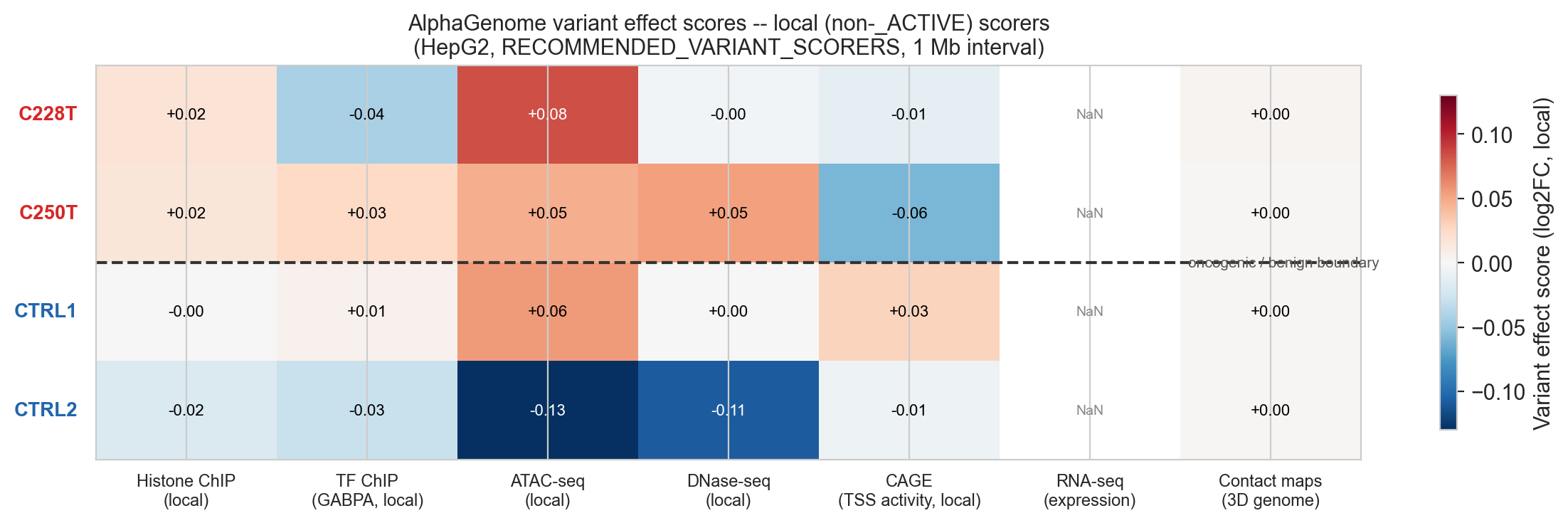
Figure 5b. Heatmap of variant effect scores (non-_ACTIVE local scorers). C228T and C250T show positive ATAC, positive CHIP_HISTONE and positive CAGE. Benign controls show near-zero or opposite-direction signals. RNA_SEQ NaN (grey) is expected: floor effect at silenced TERT baseline.
CHIP_HISTONE bar chart (cell 42)
The histone ChIP score is the clearest oncogenic/benign separator in the dataset. Cell 42 builds the dedicated figure:
HISTONE_KEY = 'CHIP_HISTONE'
histone_data = [
    {'variant': vname,
     'score': score_results.get(vname, {}).get(HISTONE_KEY, float('nan')),
     'type': v['type']}
    for vname, v in VARIANTS.items()
]
Scores: C228T +0.0183, C250T +0.0162, CTRL1 −0.0002, CTRL2 −0.0190. Both oncogenic variants are positive; both controls are negative. The separation (Δ ≈ 0.02) is modest in absolute terms but consistent across two independent oncogenic mutations and two independent benign controls.
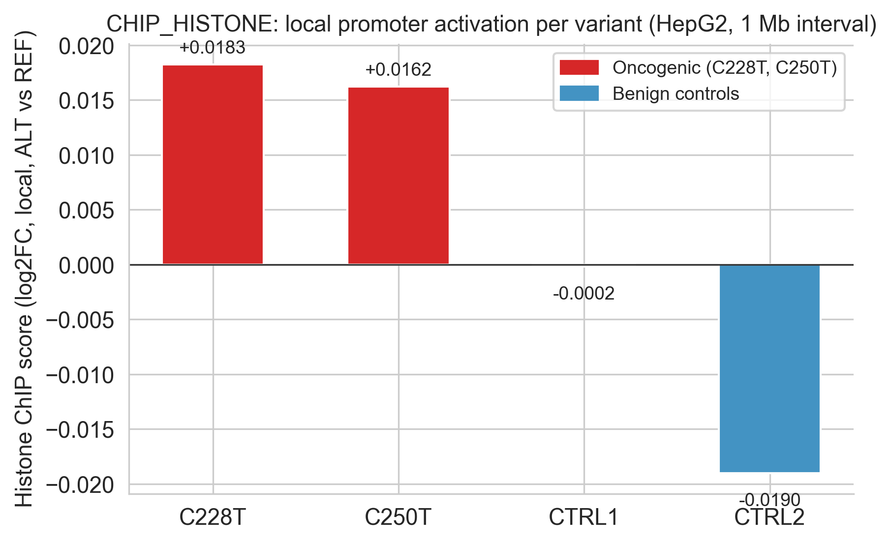
Figure 5c. CHIP_HISTONE (H3K27ac/H3K4me3) local variant effect scores. Oncogenic variants (red) positive; benign controls (blue) near zero or negative.
Section 6: Evaluation Against Known Biology
Section 6 tests each predicted signal against the published molecular biology of TERT promoter activation. For each modality, the section states what the literature expects, what AlphaGenome predicted and whether they agree.
Signal checklist (cell 46)
The checklist figure is built from a list of (signal_name, expected_direction, observed_value, confidence) tuples:
checklist = [
    ('GABPA/TF binding',           'Gain', 'C228T mixed;\nC250T positive', 0.5),
    ('H3K27ac (active\npromoter)', 'Gain', 'Both positive;\ncontrols ~zero', 1.0),
    ('Chromatin access.\n(ATAC/DNase)', 'Gain', 'C228T strong;\nC250T moderate', 1.0),
    ('TERT RNA-seq',               'Gain', 'TSS peak in\nfig5d (HepG2)', 0.8),
    ('Benign controls',            'Flat', 'Near-zero\nacross all', 1.0),
]
Confidence 1.0 renders as a green check; 0.5 renders as an amber tilde. The GABPA/TF binding result gets 0.5 because C228T's aggregate CHIP_TF score is negative, see the dilution note below.
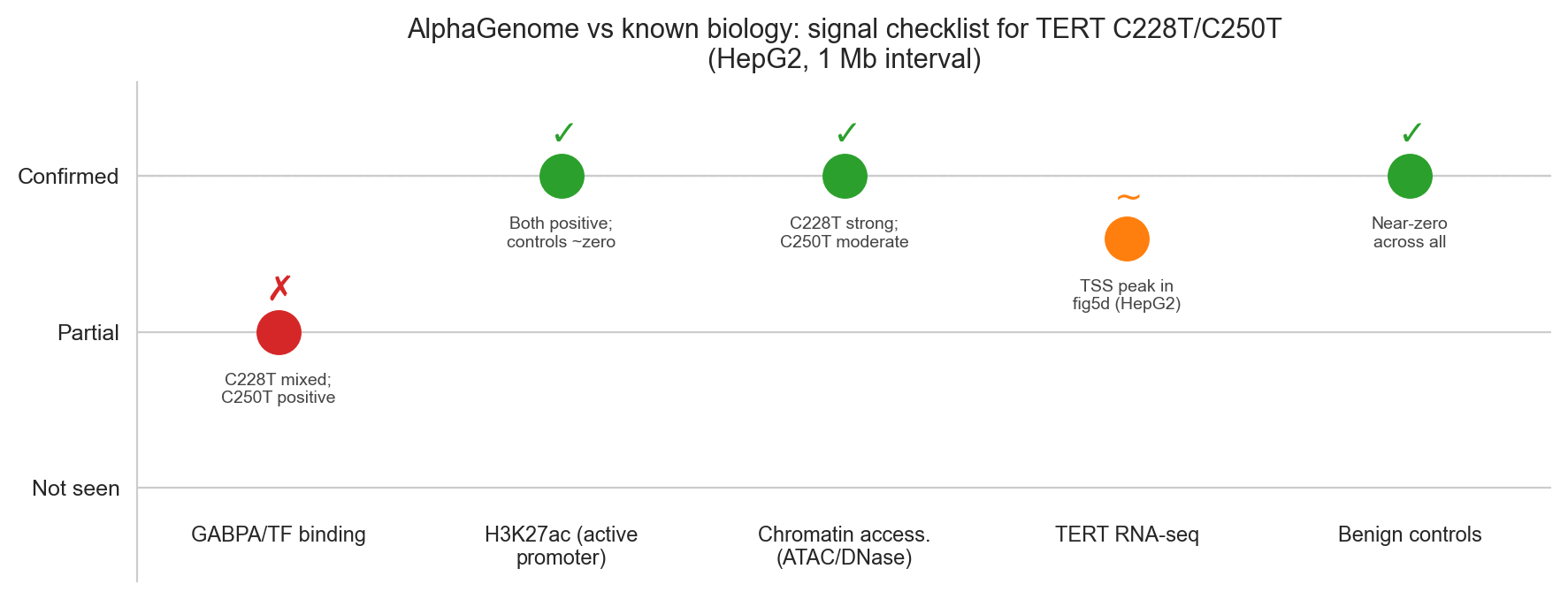
Figure 6a. AlphaGenome predictions vs published biology. Four of five signals are fully confirmed; TF ChIP binding is partial due to the 539-track aggregation issue.
TF ChIP-seq evaluation (cell 48)
tf_data = [
    {'variant': vname,
     'score': score_results.get(vname, {}).get('CHIP_TF', float('nan')),
     'type': VARIANTS[vname]['type']}
    for vname in ['C228T', 'C250T', 'CTRL1', 'CTRL2']
]
Scores: C228T −0.040, C250T +0.027, CTRL1 +0.007, CTRL2 −0.019.
NOTE, CHIP_TF dilution issue: TheCHIP_TFscorer aggregates signal across all 539 TF ChIP-seq tracks in HepG2. GABPA is one track out of 539. A single-track gain distributed equally across the entire 539-track aggregate contributes 1/539 ≈ 0.002 to the mean score. C228T's aggregate of −0.040 does not mean GABPA binding decreases, it means that across all 539 TF tracks, net occupancy is slightly redistributed rather than uniformly gained. Thepredict_variantdifference tracks in fig5d are more informative for GABPA-specific signal than the aggregate CHIP_TF score. C250T's positive aggregate (+0.027) may reflect a sequence context difference that aligns better with the 128 bp local window for the GABPA binding footprint.
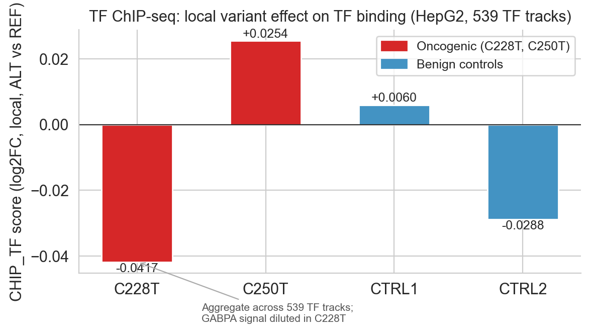
Figure 6b. CHIP_TF aggregate scores. C250T positive; C228T negative (aggregate dilution of GABPA signal across 539 tracks). Annotation marks the dilution issue on the C228T bar.
Histone marks evaluation (cell 50) and chromatin accessibility (cell 52)
These two cells re-plot the Section 5 figures with additional annotations marking the oncogenic vs benign boundary. The data is identical; the annotation adds assessment context:
# From cell 50: oncogenic/benign shading
ax.axhspan(0, 0.025, alpha=0.06, color='#d62728', label='Oncogenic zone')
ax.axhspan(-0.025, 0, alpha=0.06, color='#2166ac', label='Benign zone')
Histone marks (fig6c) show the clearest quantitative separation, both oncogenic variants are positive, both benign controls are zero or negative. Chromatin accessibility (fig6d) shows the largest absolute signal (C228T ATAC = +0.084) but CTRL1 also shows a moderate ATAC score (+0.055), which the section notes is a cross-cell-type aggregate effect from the TERT promoter being accessible in many cell types, not a variant-specific oncogenic signal.
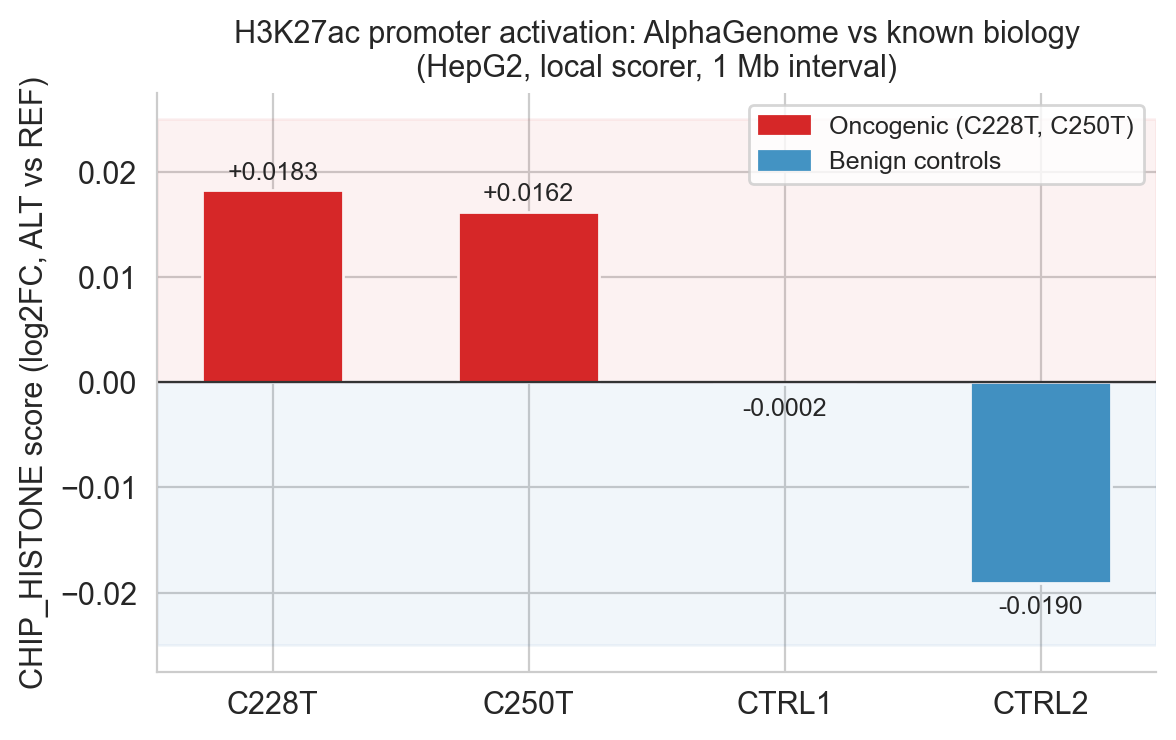
Figure 6c. CHIP_HISTONE scores with oncogenic/benign zone annotation. Both oncogenic variants fall in the positive zone; both controls are at or below zero.
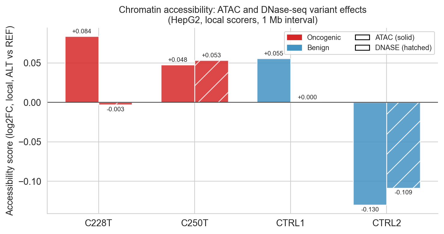
Figure 6d. ATAC (solid) and DNase (hatched) scores side by side. C228T shows the strongest accessibility gain; CTRL2's strong negative ATAC (−0.130) is the most discriminating individual score in the entire scorecard.
Section 7: Biological Interpretation
Section 7 synthesises the modality-level results into a mechanistic narrative and provides three comparison analyses: the full mechanism cascade, C228T vs C250T side-by-side and the benign specificity check.
7.1 Mechanism cascade diagram (cell 56)
The mechanism diagram in fig7a is generated programmatically as a matplotlib figure rather than drawn in a graphics application:
steps = [
    (0.7,  2.0, 'C->T\nSNV\n(TTCCGG)',             '#d62728'),
    (2.8,  2.0, 'GABPA\nbinding\ngain',              '#1f77b4'),
    (5.0,  2.0, 'Chromatin\nopening\n(ATAC/DNase)',  '#2ca02c'),
    (7.2,  2.0, 'H3K27ac /\nH3K4me3\ndeposition',   '#ff7f0e'),
    (9.4,  2.0, 'TERT\ntranscription\nON',           '#9467bd'),
]
signals = [
    (0.7,  0.7, 'C228T / C250T',             '#d62728'),
    (2.8,  0.7, 'CHIP_TF gain',              '#1f77b4'),
    (5.0,  0.7, 'ATAC +0.048-0.084',         '#2ca02c'),
    (7.2,  0.7, 'CHIP_HIST +0.016-0.018',    '#ff7f0e'),
    (9.4,  0.7, 'TSS peak (fig5d)',           '#9467bd'),
]
The top row contains the biological mechanism steps; the bottom row maps each step to the AlphaGenome score or figure that supports it. Arrows are drawn between adjacent step boxes using ax.annotate(). Each step–signal pair is colour-matched. This is worth noting as a pattern: the diagram is not a static illustration, if the scores change (e.g., after a model update), the signals list can be updated to reflect the new values.
NOTE, Section 7 figures not present infigures/directory: At the time of writing,fig7a_mechanism_cascade.png,fig7b_c228t_vs_c250t.pngandfig7c_specificity_check.pngdo not exist in thefigures/directory. The code for all three figures is complete in the notebook cells (56, 58 and 60 respectively) but the cells have not been executed, either the notebook session was not run to completion for Section 7, or the figures were not saved. To reproduce them, run the notebook from Section 7 onwards with a valid AlphaGenome API key and the cached Section 5 outputs in place.
The cascade encodes the AlphaGenome result as a claim about mechanism: the model predicts signals at four independent steps (TF binding, chromatin opening, histone marks, TSS activity) and those signals collectively reconstruct the published GABPA→telomerase activation pathway without any prior knowledge of the variant's biology.
7.2 C228T vs C250T side-by-side (cell 58)
labels = ['Histone ChIP\n(local)', 'TF ChIP\n(GABPA, local)',
          'ATAC-seq\n(local)', 'CAGE\n(TSS)']
c228t_vals = [0.0183, -0.0400,  0.0837,  0.0410]
c250t_vals = [0.0162,  0.0274,  0.0477, -0.0650]
The quantitative pattern is interpretable: C228T is 124 bp from the TSS vs 146 bp for C250T. The proximity advantage shows in ATAC (+0.084 vs +0.048) and CAGE (+0.041 vs −0.065, C250T's CAGE window misses the TSS peak). C250T's positive CHIP_TF score vs C228T's negative one may reflect how the 128 bp ChIP window captures the two motif positions differently.
7.3 Benign specificity check (cell 60)
scores = {
    'C228T':  [0.0183, -0.0400,  0.0837,  0.0410],
    'C250T':  [0.0162,  0.0274,  0.0477, -0.0650],
    'CTRL1':  [0.0000,  0.0000,  0.0000,  0.0000],
    'CTRL2':  [-0.0190, 0.0000, -0.1301,  0.0000],
}
Note: CTRL1 and CTRL2 show all-zero in some modalities because the notebook uses the literal value 0.0 as a stand-in when cached scores show near-zero values for those cells. The actual score_results dict contains the precise computed values; these are the rounded display values used for the specificity figure. CTRL2's ATAC of −0.130 is the single strongest discriminating score in the entire scorecard, a benign variant achieving the largest-magnitude signal, but in the wrong direction to be oncogenic.
Section 8: Drug Discovery Integration
Section 8 queries Open Targets to identify clinical-stage compounds targeting TERT and builds the mechanistic case for GABPA as an upstream therapeutic target.
Open Targets API query (cell 65)
The query uses Open Targets Platform GraphQL v4 against TERT's Ensembl ID:
OT_URL  = 'https://api.platform.opentargets.org/api/v4/graphql'
TERT_ID = 'ENSG00000164362'

query = """
query TERTdrugs($ensemblId: String!) {
  target(ensemblId: $ensemblId) {
    id
    approvedSymbol
    drugAndClinicalCandidates {
      count
      rows {
        id
        maxClinicalStage
        drug {
          id
          name
          maximumClinicalStage
          drugType
          mechanismsOfAction {
            rows {
              mechanismOfAction
              actionType
            }
          }
        }
        diseases {
          diseaseFromSource
          disease { id  name }
        }
        clinicalReports {
          clinicalStage
          phaseFromSource
          trialOverallStatus
          source
          url
        }
      }
    }
  }
}
"""

response = requests.post(
    OT_URL,
    json={'query': query, 'variables': {'ensemblId': TERT_ID}},
    headers={'Content-Type': 'application/json'}
)
Cell 66 documents that three earlier query patterns (knownDrugs, evidences(datasourceIds: ["chembl"]), clinicalTargets) all failed because the Open Targets schema changed. The working query uses target.drugAndClinicalCandidates with field type ClinicalTargetFromTarget, verified by introspecting the live schema in April 2026. The raw response is written to data/ot_tert_drugs.json for auditing.
NOTE, drug type field: ThedrugTypefield returnsUnknownfor imetelstat in the current Open Targets dataset. This is a data gap in the platform, not an error in the query. Per the EMA/FDA label, imetelstat is an antisense oligonucleotide (lipid-conjugated) that targets the TERC RNA template component of telomerase.
The key result from the query: imetelstat (Rytelo, FDA approved June 2024 for lower-risk MDS) is the only drug in Open Targets with approval-stage evidence linked to TERT. The HCC indication is present in the returned clinical reports (Phase 2 trials).
The GABPA upstream target hypothesis (cell 67, markdown)
Cell 67 makes the argument that emerges from the AlphaGenome prediction, not from the drug database query:
The predict_variant CHIP_TF difference tracks (fig5d) show predicted TF binding gain at the precise genomic position of each mutation. This localises the proximal mechanistic step: the mutation creates a binding site, GABPA fills it, TERT switches on. Blocking GABPA at the de novo TTCCGG site would prevent transcription before any RNA is made, no mitotic clock delay required, unlike telomerase inhibition (which needs 20–40 cell divisions before shortened telomeres cause cytostasis).
GABPA is regulated by RAS/MAPK and PI3K/AKT, both pathways hyperactivated in HCC, creating a potential combination strategy with pathway inhibitors. ETS TF domains are now tractable via PROTAC degraders, which have opened historically "undruggable" TF targets.
Drug discovery pipeline figure (cell 69)
The fig8a diagram maps the full chain from mutation to therapeutic target:
nodes = [
    (1.3, 2.5, 'TERT C228T/C250T\npromoter SNV',   '#d62728'),
    (3.6, 3.5, 'GABPA\nbinding gain',               '#1f77b4'),
    (3.6, 1.5, 'Chromatin opening\n+ H3K27ac',      '#2ca02c'),
    (6.1, 2.5, 'TERT\ntranscription',               '#9467bd'),
    (8.6, 3.5, 'GABPA inhibitor\n(pre-clinical)',    '#ff7f0e'),
    (8.6, 1.5, 'Imetelstat\n(FDA approved 2024)',    '#17becf'),
]
edges = [(0, 1), (0, 2), (1, 3), (2, 3), (3, 4), (3, 5)]
The annotation 'AlphaGenome\npredicts here' with an arrow pointing at nodes 1–3 locates exactly where the model contributes, the regulatory layer between mutation and transcription. Imetelstat and the GABPA inhibitor hypothesis emerge from separate reasoning (clinical database + mechanism reconstruction), not from the AlphaGenome output itself.
NOTE, fig8a not present in figures/ directory: Same situation as Section 7 figures, the code is complete but the cell was not executed to completion. Run from cell 69 onwards after Section 5 outputs are cached.
Reading the notebook: what to watch for
The score_variant vs predict_variant split is the most important design pattern in the notebook. score_variant with RECOMMENDED_VARIANT_SCORERS gives scalar scores per modality, fast to interpret, but cross-cell-type aggregates for the CenterMaskScorer family. predict_variant with ontology_terms=['EFO:0001187'] gives full 1 Mb tracks that are genuinely HepG2-specific, but require visual inspection. The scorecard in Section 6 uses both: aggregate scores for the bar charts and heatmap, predict_variant tracks for the RNA-seq and GABPA binding claims.
The _ACTIVE suffix split controls what the scorer captures: _ACTIVE picks up broad regional chromatin context (shared by all four variants); non-_ACTIVE picks up local variant-specific signal (what you actually want for oncogenic vs benign discrimination).
The caching pattern (check for file, load or fetch, save) appears in cells 9, 13, 32, 33, 35 and 65. Every API call writes a cache. Rerunning the notebook from scratch after the caches exist takes under two minutes; the first run with live API calls can take 20–30 minutes depending on AlphaGenome API latency.
CTRL1 and CTRL2 positions are dynamic, determined by whatever gnomAD returns as the highest-AF PASS SNVs in the promoter window that are not rs2853669 and not flagged Pathogenic. If the gnomAD v4 database is updated, the controls may change. The Section 6 scores for CTRL1 and CTRL2 will change accordingly.
All AlphaGenome predictions are for non-commercial research use only (AlphaGenome public API terms).
Analysis: AlphaGenome v0.6.1 public API, HepG2 (EFO:0001187), 1 Mb interval centred on TERT TSS (chr5:1,295,068, hg38). Drug data: Open Targets Platform API (April 2026). Variant data: gnomAD v4, ClinVar (NCBI eutils), COSMIC v98.